https://medium.com/towards-data-science/parallelize-your-massive-shap-computations-with-mllib-and-pyspark-b00accc8667c
(能翻墙直接看原文)
A stepwise guide for efficiently explaining your models using SHAP.

Photo by Pietro Jeng on Unsplash
Introduction to MLlib
Apache Spark’s Machine Learning Library (MLlib) is designed primarily for scalability and speed by leveraging the Spark runtime for common distributed use cases in supervised learning like classification and regression, unsupervised learning like clustering and collaborative filtering and in other cases like dimensionality reduction. In this article, I cover how we can use SHAP to explain a Gradient Boosted Trees (GBT) model that has fit our data at scale.
What are Gradient Boosted Trees?
Before we understand what Gradient Boosted Trees are, we need to understand boosting. Boosting is an ensemble technique that sequentially combines a number of weak learners to achieve an overall strong learner. In case of Gradient Boosted Trees, each weak learner is a decision tree that sequentially minimizes the errors (MSE in case of regression and log loss in case of classification) generated by the previous decision tree in that sequence. To read about GBTs in more detail, please refer to this blog post.
Understanding our imports
from pyspark.sql import SparkSession
from pyspark import SparkContext, SparkConf
from pyspark.ml.classification import GBTClassificationModel
import shap
import pyspark.sql.functions as F
from pyspark.sql.types import *
The first two imports are for initializing a Spark session. It will be used for converting our pandas dataframe to a spark one. The third import is used to load our GBT model into memory which will be passed to our SHAP explainer to generate explanations. The SHAP explainer itself will be initialized using the SHAP package using the fourth import. The penultimate and last import is for performing SQL functions and using SQL types. These will be used in our User-Defined Function (UDF) which I shall describe later.
Converting our MLlib GBT feature vector to a Pandas dataframe
The SHAP Explainer takes a dataframe as input. However, training an MLlib GBT model requires data preprocessing. More specifically, the categorical variables in our data needs to be converted into numeric variables using either Category Indexing or One-Hot Encoding. To learn more about how to train a GBT model, refer to this article). The resulting “features” column is a SparseVector (to read more on it, check the “Preprocess Data” section in this example). It looks like something below:

SparseVector features column description — 1. default index value, 2. vector length, 3. list of indexes of the feature columns, 4. list of data values at the corresponding index at 3. [Image by author]
The “features” column shown above is for a single training instance. We need to transform this SparseVector for all our training instances. One way to do it is to iteratively process each row and append to our pandas dataframe that we will feed to our SHAP explainer (ouch!). There is a much faster way, which leverages the fact that we have all of our data loaded in memory (if not, we can load it in batches and perform the preprocessing for each in-memory batch). In Shikhar Dua’s words:
1. Create a list of dictionaries in which each dictionary corresponds to an input data row.
2. Create a data frame from this list.
So, based on the above method, we get something like this:
rows_list = []
for row in spark_df.rdd.collect():
    dict1 = {}
    dict1.update({k:v for k,v in zip(spark_df.cols,row.features)})
    rows_list.append(dict1)
pandas_df = pd.DataFrame(rows_list)
If rdd.collect() looks scary, it’s actually pretty simple to explain. Resilient Distributed Datasets (RDD) are fundamental Spark data structures that are an immutable distribution of objects. Each dataset in an RDD is further subdivided into logical partitions that can be computed in different worker nodes of our Spark cluster. So, all PySpark RDD collect() does is retrieve data from all the worker nodes to the driver node. As you might guess, this is a memory bottleneck, and if we are handling data larger than our driver node’s memory capacity, we need to increase the number of our RDD partitions and filter them by partition index. Read how to do that here.
Don’t take my word on the execution performance. Check out the stats.
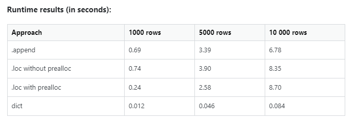
Performance profiling for inserting rows to a pandas dataframe. [Source (Thanks to Mikhail_Sam and Peter Mortensen): here]
Here are the metrics from one of my Databricks notebook scheduled job runs:
Input size: 11.9 GiB (~12.78GB), Total time Across All Tasks: 20 min, Number of records: 165.16K
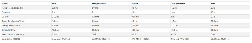
Summary Metrics for 125 Completed Tasks executed by the stage that run the above cell. [Image by author]
Working with the SHAP Library
We are now ready to pass our preprocessed dataset to the SHAP TreeExplainer. Remember that SHAP is a local feature attribution method that explains individual predictions as an algebraic sum of the shapley values of the features of our model.
We use a TreeExplainer for the following reasons:
- Suitable: TreeExplainer is a class that computes SHAP values for tree-based models (Random Forest, XGBoost, LightGBM, GBT, etc).
- Exact: Instead of simulating missing features by random sampling, it makes use of the tree structure by simply ignoring decision paths that rely on the missing features. The TreeExplainer output is therefore deterministic and does not vary based on the background dataset.
- Efficient: Instead of iterating over each possible feature combination (or a subset thereof), all combinations are pushed through the tree simultaneously, using a more complex algorithm to keep track of each combination’s result — reducing complexity from O(TL2ᵐ) for all possible coalitions to the polynomial O(TLD²) (where m is the number of features, T is number of trees, L is maximum number of leaves and D is maximum tree depth).
The check_additivity = False flag runs a validation check to verify if the sum of SHAP values equals to the output of the model. However, this flag requires predictions to be run that are not supported by Spark, so it needs to be set to False as it is ignored anyway. Once we get the SHAP values, we convert it into a pandas dataframe from a Numpy array, so that it is easily interpretable.
One thing to note is that the dataset order is preserved when we convert a Spark dataframe to pandas, but the reverse is not true.
The points above lead us to the code snippet below:
gbt = GBTClassificationModel.load('your-model-path')
explainer = shap.TreeExplainer(gbt)
shap_values = explainer(pandas_df, check_additivity = False)
shap_pandas_df = pd.DataFrame(shap_values.values, cols = pandas_df.columns)
An Introduction to Pyspark UDFs and when to use them

How PySpark UDFs distribute individual tasks to worker (executor) nodes [Source: here]
User-Defined Functions are complex custom functions that operate on a particular row of our dataset. These functions are generally used when the native Spark functions are not deemed sufficient to solve the problem. Spark functions are inherently faster than UDFs because it is natively a JVM structure whose methods are implemented by local calls to Java APIs. However, PySpark UDFs are Python implementations that requires data movement between the Python interpreter and the JVM (refer to Arrow 4 in the picture above). This inevitably introduces some processing delay.
If no processing delays can be tolerated, the best thing to do is create a Python wrapper to call the Scala UDF from PySpark itself. A great example is shown in this blog. However, using a PySpark UDF was sufficient for my use case, since it is easy to understand and code.
The code below explains the Python function to be executed on each worker/executor node. We just pick up the highest SHAP values (absolute values as we want to find the most impactful negative features as well) and append it to the respective pos_features and neg_features list and in turn append both these lists to a features list that is returned to the caller.
def shap_udf(row):
    dict = {}
    pos_features = []
    neg_features = []
    for feature in row.columns:
        dict[feature] = row[feature]     dict_importance = {key: value for key, value in
    sorted(dict.items(), key=lambda item: __builtin__.abs(item[1]),
    reverse = True)}     for k,v in dict_importance.items():
        if __builtin__.abs(v) >= <your-threshold-shap-value>:
             if v > 0:
                 pos_features.append((k,v))
             else:
                 neg_features.append((k,v))
   features = []
   features.append(pos_features[:5])
   features.append(neg_features[:5])    return features
We then register our PySpark UDF with our Python function name (in my case, it is shap_udf) and specify the return type (mandatory in Python and Java) of the function in the parameters to F.udf(). There are two lists in the outer ArrayType(), one for positive features and the other for negative ones. Since each individual list comprises of at most 5 (feature-name, shap-value) StructType() pairs, it represents the inner ArrayType(). Below is the code:
udf_obj = F.udf(shap_udf, ArrayType(ArrayType(StructType([ StructField(‘Feature’, StringType()),
StructField(‘Shap_Value’, FloatType()),
]))))
Now, we just create a new Spark dataframe with a column called ‘Shap_Importance’ that invokes our UDF for each row of the spark_shapdf dataframe. To split the positive and negative features, we create two columns in a new Spark dataframe called final_sparkdf. Our final code-snippet looks like below:
new_sparkdf = spark_df.withColumn(‘Shap_Importance’, udf_obj(F.struct([spark_shapdf[x] for x in spark_shapdf.columns])))final_sparkdf = new_sparkdf.withColumn(‘Positive_Shap’, final_sparkdf.Shap_Importance[0]).withColumn(‘Negative_Shap’, new_sparkdf.Shap_Importance[1])
And finally, we have extracted all the important features of our GBT model per testing instance without the use of any explicit for loops! The consolidated code can be found in the below GitHub gist.
from pyspark.sql import SparkSession
from pyspark import SparkContext, SparkConf
from pyspark.ml.classification import GBTClassificationModel
import shap
import pyspark.sql.functions as  F
from pyspark.sql.types import *

#convert the sparse feature vector that is passed to the MLlib GBT model into a pandas dataframe.
#This 'pandas_df' will be passed to the Shap TreeExplainer.
rows_list = []
for row in spark_df.rdd.collect():
  dict1 = {}
  dict1.update({k:v for k,v in zip(spark_df.cols,row.features)})
  rows_list.append(dict1)

pandas_df = pd.DataFrame(rows_list)

#Load the GBT model from the path you have saved it
gbt = GBTClassificationModel.load("<your path where the GBT model is loaded>")
#make sure the application where your notebook runs has access to the storage path!

explainer = shap.TreeExplainer(gbt)
#check_additivity requires predictions to be run that is not supported by spark [yet], so it needs to be set to False as it is ignored anyway.
shap_values = explainer(pandas_df, check_additivity = False)
shap_pandas_df = pd.DataFrame(shap_values.values, cols = pandas_df.columns)

spark = SparkSession.builder.config(conf=SparkConf().set("spark.master", "local[*]")).getOrCreate()
spark_shapdf = spark.createDataFrame(shap_pandas_df)


def shap_udf(row): #work on a single spark dataframe row, for all rows. This work is distributed among all the worker nodes of your Apache Spark cluster.
  dict = {}
  pos_features = []
  neg_features = []

  for feature in row.columns:
    dict[feature] = row[feature]

  dict_importance = {key: value for key, value in sorted(dict.items(), key=lambda item: __builtin__.abs(item[1]), reverse = True)}

  for k,v in dict_importance.items():
    if __builtin__.abs(v) >= <your-threshold-shap-value>:
      if v > 0:
        pos_features.append((k,v))
      else:
        neg_features.append((k,v))
  features = []
  #taking top 5 features from pos and neg features. We can increase this number.
  features.append(pos_features[:5])
  features.append(neg_features[:5])

  return features


udf_obj = F.udf(shap_udf, ArrayType(ArrayType(StructType([
  StructField('Feature', StringType()),
  StructField('Shap_Value', FloatType()),
]))))

new_sparkdf = spark_df.withColumn('Shap_Importance', udf_obj(F.struct([spark_shapdf[x] for x in spark_shapdf.columns])))
final_sparkdf = new_sparkdf.withColumn('Positive_Shap', final_sparkdf.Shap_Importance[0]).withColumn('Negative_Shap', new_sparkdf.Shap_Importance[1])
Get the most impactful Positive and Negative SHAP values from our fitted GBT Model
P.S. This is my first attempt at writing an article and if there are any factual or statistical inconsistencies, please reach out to me and I shall be more than happy to learn together with you! :)
References
[1] Soner Yıldırım, Gradient Boosted Decision Trees-Explained (2020), Towards Data Science
[2] Susan Li, Machine Learning with PySpark and MLlib — Solving a Binary Classification Problem (2018), Towards Data Science
[3] Stephen Offer, How to Train XGBoost With Spark (2020), Data Science and ML
[4] Use Apache Spark MLlib on Databricks (2021), Databricks
[5] Umberto Griffo, Don’t collect large RDDs (2020), Apache Spark — Best Practices and Tuning
[6] Nikhilesh Nukala, Yuhao Zhu, Guilherme Braccialli, Tom Goldenberg (2019), Spark UDF — Deep Insights in Performance, QuantumBlack


![[DDR4] DDR 简史](https://img-blog.csdnimg.cn/direct/8d31fad7a28745eb81e253606f226423.png#pic_center)

![[vue3]组件通信](https://img-blog.csdnimg.cn/img_convert/014c79cb2027c4c5a84dd8760b1035de.png)